How to Predict Sales in Microsoft Fabric


It feels like an eternity since I last wrote a technical walkthrough! I managed to get some downtime to try some sandbox Data Science workflows in Microsoft Fabric that I want to share with you.
In his scenario I want to build a sales forecasting model to predict product sales quantites for a specific customer.
Throughout my career I have witnessed firsthand how powerful Forecasting is in sales. The approach we will take today combines historical data and predictive methods to provide insights into future trends. Forecasting can analyse past sales to identify patterns, and learn from consumer behavior to optimise inventory, production, and marketing strategies.
What This Walkthrough Covers
In this walkthrough, we will cover the following steps:
-
Loading the historic data
-
Use exploratory data analysis to understand and process the data
-
Train a machine learning model with an open-source software package, and track experiments
-
Save the final machine learning model, and make predictions
-
Show the model performance with Python visualisations
Setting Up the Environment
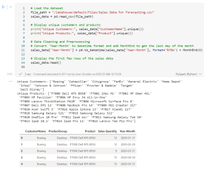
In this scenario, we have preloaded historic sales data for companies purchasing electronic equipment via csv file format into the Lakehouse within Fabric.
To begin let’s install and load the required libraries in Python.
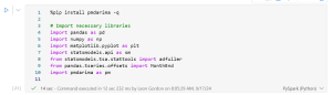
Install and Import Required Libraries
Loading and Transforming the Data
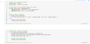
Next we will load the data into a pandas data frame and explore the data to identify unique customers and products within the dataset. This will later be used to support selecting a customer and product pairing to analyse and forecast product purchasing.
We then need to make some small transformations on the dataset, aggregating the data to the month level.
 Load and Transform the Data
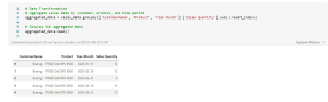 Aggregate the Data
Filtering to a Customer and Product
Next, we can filter the contents of the data frame showing a single customer “Boeing” and their historic sales quantities for the “P700 Dell XPS 8950” product, we will programatically check if relevant data is available for the specified customer and product combination,. This historic dataset will form the base for our analysis.
Filter Data to Specified Customer and Product
Exploring Trends and Seasonality
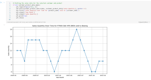
We can now start to perform some trend analysis, firstly, we can plot the sales data using Matplotlib. We visualise the sales quantity over time for the specified customer and product. This time series plot helps identify trends, patterns, and any irregularities in the sales data.
We then conduct the Augmented Dickey-Fuller (ADF) test to check if the sales data is stationary. Stationarity is a key assumption for many time series forecasting models, and the ADF test statistically determines if the time series has a constant mean and variance over time.
Finally, we break down the sales data into trend, seasonal, and residual components. The goal of this analysis is to reveal underlying patterns such as recurring seasonal effects and long-term trends, which are crucial for building an accurate forecasting model.
 Visualising Sales Quantity Over Time
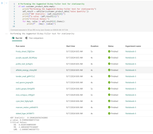 Augmented Dickey-Fuller (ADF) Test
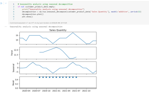 Seasonality Analysis Using Seasonal Decomposition
Building the SARIMA Model
Next we will focus on building a Seasonal ARIMA (SARIMA) model to forecast sales quantities.
To do this we configure the model with auto_arima. The auto_arima function from the pmdarima library is great as it allows us to automate the process of finding the optimal SARIMA model parameters. This function tests different combinations of ARIMA orders to identify the best fit based on statistical criteria.
By fitting a SARIMA model, we aim to capture both the non-seasonal and seasonal patterns in the sales data, providing a robust tool for making accurate sales forecasts.
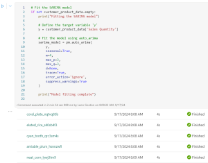 Fitting the Model
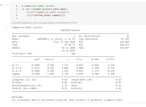
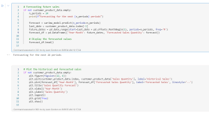
Forecasting Future Sales
In this final part of this walkthrough, we will use the trained SARIMA model to forecast future sales quantities for the next 24 months.
We call the predict method on the sarima_model to forecast sales for the next 24 periods (e.g., months).
By generating these predictions, we will complete the most powerful aspect of the sales forecasting process using the SARIMA model.
This final visual can be utilised for many business goals including enabling the business to anticipate future sales trends for the selected customer and product, aiding in strategic planning and resource allocation.
 Forecasting Future Sales Quantity
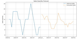
Wrap-Up and Next Steps
We’ve now explored the foundational steps for predicting sales using Microsoft Fabric.
Starting with data visualisation and exploratory analysis, we’ve identified trends, seasonality, and patterns within our sales data.
We’ve also prepared our data for modeling by testing for stationarity and decomposing the time series to understand its underlying components.
While we’ve set up the SARIMA model and generated initial forecasts, this guide serves as an introduction rather than a comprehensive solution and can be expanded upon in multiple ways
In future posts I would like to explore:
-
Model Fitting and Fine-Tuning
-
Model Evaluation and Comparison in Fabric
-
Deployment of the ML Model in Microsoft Fabric
-
Automating Prediction for Multiple Customers and Products
This journey is an ongoing process of learning and improvement. By continuously refining the model and leveraging the capabilities of Microsoft Fabric, you can develop a robust sales forecasting system that provides valuable insights and supports data-driven decision-making.
Thank you for following along, and I look forward to exploring this further with you in future walkthroughs!
Written by Leon Gordon
Related Articles